Getting Started with supremo_lite
Introduction to core functionality for generating personalized genome sequences and variant-centered windows.
What is supremo_lite?
supremo_lite is a lightweight Python package for:
Generating personalized genome sequences from reference genomes and variant files
Creating variant-centered sequence windows for model predictions
Performing in-silico saturation mutagenesis
Aligning predictions across reference and variant sequences
Designed to be memory-efficient and model-agnostic, supporting both PyTorch tensors and NumPy arrays.
Installation
If you haven’t already installed supremo_lite:
pip install supremo-lite
Basic Imports
import supremo_lite as sl
import numpy as np
import matplotlib.pyplot as plt
from pyfaidx import Fasta
import pandas as pd

print(f"supremo_lite version: {sl.__version__}")

## Optional packages:

# Check PyTorch availability
print(f"PyTorch available: {sl.TORCH_AVAILABLE}")

# Check brisket availability (faster 1h encoding)
print(f"brisket available: {sl.BRISKET_AVAILABLE}")
supremo_lite version: 1.0.0
PyTorch available: True
brisket available: True
DNA Sequence Encoding
supremo_lite uses one-hot encoding: A=[1,0,0,0], C=[0,1,0,0], G=[0,0,1,0], T=[0,0,0,1].
Functions automatically return PyTorch tensors when available, otherwise NumPy arrays.
Loading Test Data
For this tutorial, we’ll use small test data included with the package. This allows for quick demonstrations without requiring large genomic datasets.
import os

# Find the test data directory
# Assuming we're in the package directory structure
test_data_dir = "../../tests/data"

# Load reference genome
reference_path = os.path.join(test_data_dir, "test_genome.fa")
reference = Fasta(reference_path)

print("Reference genome chromosomes:")
for chrom in reference.keys():
    seq_len = len(reference[chrom])
    print(f"  {chrom}: {seq_len} bp")

# Show first 80 bp of chr1
print(f"\nchr1 sequence (first 80 bp):")
print(reference["chr1"][:80].seq)
Reference genome chromosomes:
  chr1: 80 bp
  chr2: 80 bp
  chr3: 80 bp
  chr4: 80 bp
  chr5: 80 bp
  chr6: 80 bp

chr1 sequence (first 80 bp):
ATGAATATAATATTTTCGAGAATTACTCCTTTTGGAAATGGAACATTATGCGTTTTAAGAGTTTCTGGTAACAATATATT
Reading VCF Files
supremo_lite provides utilities to read VCF (Variant Call Format) files:
# Load SNP variants
snp_vcf_path = os.path.join(test_data_dir, "snp", "snp.vcf")
snp_variants = sl.read_vcf(snp_vcf_path)

print("SNP variants:")
print(snp_variants)
print(f"\nLoaded {len(snp_variants)} SNP variant(s)")
SNP variants:
  chrom  pos1 id ref alt    info  vcf_line variant_type
0  chr1     2  .   T   G  DP=100         8          SNV
1  chr1    31  .   T   A  DP=100         9          SNV
2  chr2    19  .   A   G  DP=100        10          SNV
3  chr2    57  .   C   G  DP=100        11          SNV

Loaded 4 SNP variant(s)
Basic Usage: Creating a Personalized Genome
The most fundamental operation is applying variants to a reference genome to create a personalized genome:
# Create personalized genome (returns encoded sequences by default)
personal_genome = sl.get_personal_genome(
    reference_fn=reference,
    variants_fn=snp_variants,
    encode=True,
    verbose=True,  # Show progress
)

# Check the result
print(f"\nPersonalized genome chromosomes: {list(personal_genome.keys())}")
print(f"chr1 encoded shape: {personal_genome['chr1'].shape}")
print(f"Data type: {type(personal_genome['chr1'])}")
🧬 Processing 4 variants across 2 chromosomes
   Phase 1: 4 standard variants (SNV, MNV, INS, DEL, SV_DUP, SV_INV)
   Phase 2: 0 BND variants for semantic classification
🔄 Processing chromosome chr1: 2 variants (2 SNV)
  ✅ Applied 2/2 variants (0 skipped)
🔄 Processing chromosome chr2: 2 variants (2 SNV)
  ✅ Applied 2/2 variants (0 skipped)
🧬 Completed: 4/4 variants processed → 6 sequences

Personalized genome chromosomes: ['chr1', 'chr2', 'chr3', 'chr4', 'chr5', 'chr6']
chr1 encoded shape: torch.Size([4, 80])
Data type: <class 'torch.Tensor'>
Getting Raw Sequence Strings
You can also get the sequences as strings instead of encoded arrays:
# Get raw sequences
personal_genome_raw = sl.get_personal_genome(
    reference_fn=reference, variants_fn=snp_variants, encode=False
)

# Compare reference and personalized sequences
ref_seq = reference["chr1"][:80].seq
pers_seq = personal_genome_raw["chr1"][:80]

print("Reference chr1 (first 80 bp):")
print(ref_seq)
print("\nPersonalized chr1 (first 80 bp):")
print(pers_seq)

# Highlight the difference
print("\nDifferences (position: ref → alt):")
for i, (r, p) in enumerate(zip(ref_seq, pers_seq)):
    if r != p:
        print(f"  Position {i}: {r} → {p}")
Reference chr1 (first 80 bp):
ATGAATATAATATTTTCGAGAATTACTCCTTTTGGAAATGGAACATTATGCGTTTTAAGAGTTTCTGGTAACAATATATT

Personalized chr1 (first 80 bp):
AGGAATATAATATTTTCGAGAATTACTCCTATTGGAAATGGAACATTATGCGTTTTAAGAGTTTCTGGTAACAATATATT

Differences (position: ref → alt):
  Position 1: T → G
  Position 30: T → A
Generating Variant-Centered Windows
Often you want to extract sequence windows centered on each variant, which is useful for model predictions:
# Generate windows around variants
# Note: get_alt_ref_sequences is a generator that yields chunks
results = list(
    sl.get_alt_ref_sequences(
        reference_fn=reference,
        variants_fn=snp_variants,
        seq_len=40,  # 40 bp windows
        encode=False,  # Get strings for visualization
    )
)

# Unpack from the first chunk
alt_seqs, ref_seqs, metadata = results[0]

print(f"Generated {len(metadata)} sequence pair(s)")
print("\nMetadata:")
print(metadata.head())  # Show first few variants

print("\nReference sequence (2nd variant):")
print(ref_seqs[1])
print("\nAlternate sequence (2nd variant):")
print(alt_seqs[1])

# Find the variant position in the window
variant_offset = len(ref_seqs[1][3]) // 2
print(f"\nVariant is centered at position {variant_offset} in the window")
print(f"Reference allele: {ref_seqs[1][3][variant_offset]}")
print(f"Alternate allele: {alt_seqs[1][3][variant_offset]}")
Generated 4 sequence pair(s)

Metadata:
  chrom  window_start  window_end  variant_pos0  variant_pos1 ref alt  \
0  chr1             0          40             1             2   T   G
1  chr1            10          50            30            31   T   A
2  chr2             0          40            18            19   A   G
3  chr2            36          76            56            57   C   G

  variant_type
0          SNV
1          SNV
2          SNV
3          SNV

Reference sequence (2nd variant):
('chr1', np.int64(10), np.int64(50), 'TATTTTCGAGAATTACTCCTTTTGGAAATGGAACATTATG')

Alternate sequence (2nd variant):
('chr1', np.int64(10), np.int64(50), 'TATTTTCGAGAATTACTCCTATTGGAAATGGAACATTATG')

Variant is centered at position 20 in the window
Reference allele: T
Alternate allele: A
Sequence Utilities
supremo_lite provides useful utilities for working with DNA sequences:
# Reverse complement
sequence = "ATCGATCG"
rc_sequence = sl.rc_str(sequence)

print(f"Original:          {sequence}")
print(f"Reverse complement: {rc_sequence}")

# Encode and decode
encoded = sl.encode_seq(sequence)  # Automatically uses brisket if installed
decoded = sl.decode_seq(encoded)

print(f"\nDecoded matches original: {decoded == sequence}")

# Reverse complement of encoded sequence
rc_encoded = sl.rc(encoded)
rc_decoded = sl.decode_seq(rc_encoded)

print(f"RC from encoded:   {rc_decoded}")
print(f"RC from string:    {rc_sequence}")
print(f"Match: {rc_decoded == rc_sequence}")
Original:          ATCGATCG
Reverse complement: CGATCGAT

Decoded matches original: True
RC from encoded:   CGATCGAT
RC from string:    CGATCGAT
Match: True
Working with Encoded Sequences
Let’s see how to work with encoded sequences for downstream analysis:
# Generate encoded windows
results = list(
sl.get_alt_ref_sequences(
reference_fn=reference,
variants_fn=snp_variants,
seq_len=40,
encode=True, # Get encoded arrays/tensors
)
)
# Unpack from the first chunk
alt_seqs_enc, ref_seqs_enc, metadata = results[0]
print(f"Reference sequences shape: {ref_seqs_enc.shape}")
print(f"Alternate sequences shape: {alt_seqs_enc.shape}")
print(f"Data type: {type(ref_seqs_enc)}")
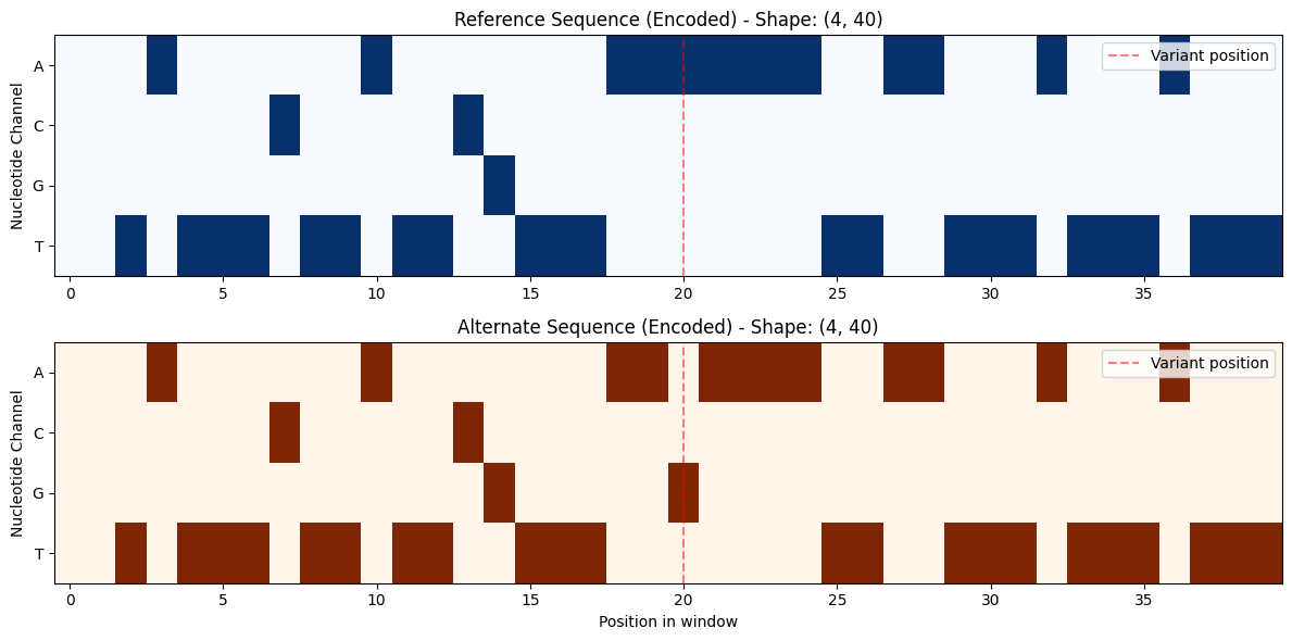
# Visualize the first sequence pair
fig, (ax1, ax2) = plt.subplots(2, 1, figsize=(12, 6))
# Convert to numpy if needed for visualization
ref_viz = (
ref_seqs_enc[2].numpy() if hasattr(ref_seqs_enc[2], "numpy") else ref_seqs_enc[2]
)
alt_viz = (
alt_seqs_enc[2].numpy() if hasattr(alt_seqs_enc[2], "numpy") else alt_seqs_enc[2]
)
# Reference sequence - data is already in (4, L) format
im1 = ax1.imshow(ref_viz, cmap="Blues", aspect="auto")
ax1.set_yticks([0, 1, 2, 3])
ax1.set_yticklabels(["A", "C", "G", "T"])
ax1.set_title("Reference Sequence (Encoded) - Shape: (4, 40)")
ax1.set_ylabel("Nucleotide Channel")
ax1.axvline(x=20, color="red", linestyle="--", alpha=0.5, label="Variant position")
ax1.legend()
# Alternate sequence - data is already in (4, L) format
im2 = ax2.imshow(alt_viz, cmap="Oranges", aspect="auto")
ax2.set_yticks([0, 1, 2, 3])
ax2.set_yticklabels(["A", "C", "G", "T"])
ax2.set_title("Alternate Sequence (Encoded) - Shape: (4, 40)")
ax2.set_xlabel("Position in window")
ax2.set_ylabel("Nucleotide Channel")
ax2.axvline(x=20, color="red", linestyle="--", alpha=0.5, label="Variant position")
ax2.legend()
plt.tight_layout()
plt.show()
print("\nThe variant at position 20 shows different encoding between ref and alt")
print(
"Note: Sequences are encoded in channel-first format (4, L) for compatibility with PyTorch models"
)
Reference sequences shape: torch.Size([4, 4, 40])
Alternate sequences shape: torch.Size([4, 4, 40])
Data type: <class 'torch.Tensor'>
The variant at position 20 shows different encoding between ref and alt
Note: Sequences are encoded in channel-first format (4, L) for compatibility with PyTorch models
Next Steps
Continue with the other notebooks:
02_personalized_genomes.ipynb - Genome personalization workflows
03_prediction_alignment.ipynb - Model predictions and alignment